
Setup: USD/JPY, intraday data. A Kalman-filter momentum rule, long and short (market-neutral). Development window 2014-2018, out-of-sample 2018-2026 held out strictly. Transaction costs of 0.2 bps included throughout. Engine: Manifold-bt.
1. A single parameter set is a noisy estimator
Consider a strategy with a few knobs, a Kalman-filter momentum rule on USD/JPY (it goes with the trend when price stretches above its Kalman-estimated level). The strategy takes long and short positions, its beta to the yen is near zero. It is a market-neutral edge. The knobs are the filter reactivity q, the lookback w and the entry threshold en. We sweep the parameters on the development window and keep one.
A careful practitioner does not keep the raw in-sample champion, whose overfitting is notorious. They keep the stable parameter set, the one whose neighbours also work, sitting on a plateau rather than a spike. Out-of-sample (2018-2026), this best stable set posts a Sharpe of 0.44, in the same range as buy and hold (0.46). The comparison is only indicative, the strategy being market-neutral and buy and hold directional.
But that figure is a single measurement. The standard error of an annualized Sharpe estimated over T years is about √((1 + ½·S²)/T). Over the 8.5 out-of-sample years it approaches 0.36. A Sharpe of 0.44 ± 0.36 has a t-stat around 1.3, below the usual 1.96 threshold. The measurement is not reliably distinguishable from zero, let alone from its neighbours.
2. The in-sample ranking does not predict out-of-sample
The crux. Plotting, for each parameter set, its in-sample Sharpe against its out-of-sample Sharpe :
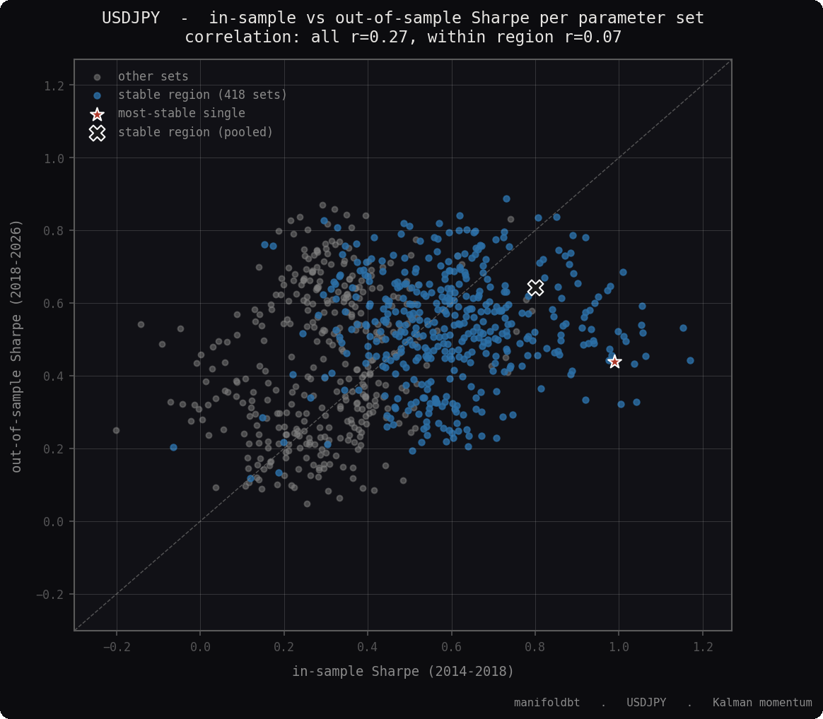
Each point is a parameter set. Within the stable region, the in-sample / out-of-sample correlation is essentially zero.
Within the relevant region the correlation is essentially nil (r ≈ 0.07). Across the whole grid a weak correlation remains (r ≈ 0.27), driven by the degenerate corners where the strategy fails in-sample and out-of-sample alike. But where you actually choose your parameters, it vanishes. This is not a prediction failure. The Sharpe gaps between plateau sets are noise, not signal. They all estimate the same underlying edge, and the in-sample ranking merely orders random realizations. The top set is not better, it is luckier, and its out-of-sample figure is just another draw.
3. The plateau: one edge, many parameterizations
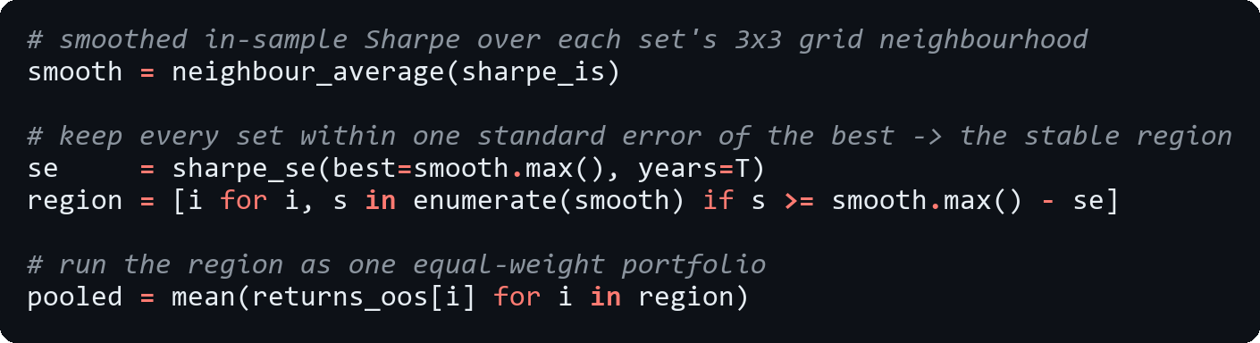
Running that sweep takes only a few lines :
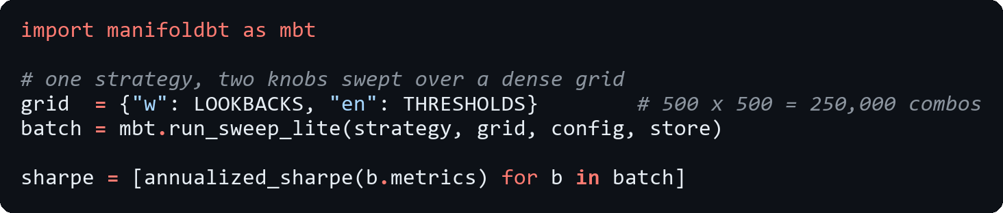
So read the shape of the surface, not its argmax. The Sharpe over the lookback × threshold grid, in-sample on the left, out-of-sample on the right, same colour scale (250,000 backtests) :
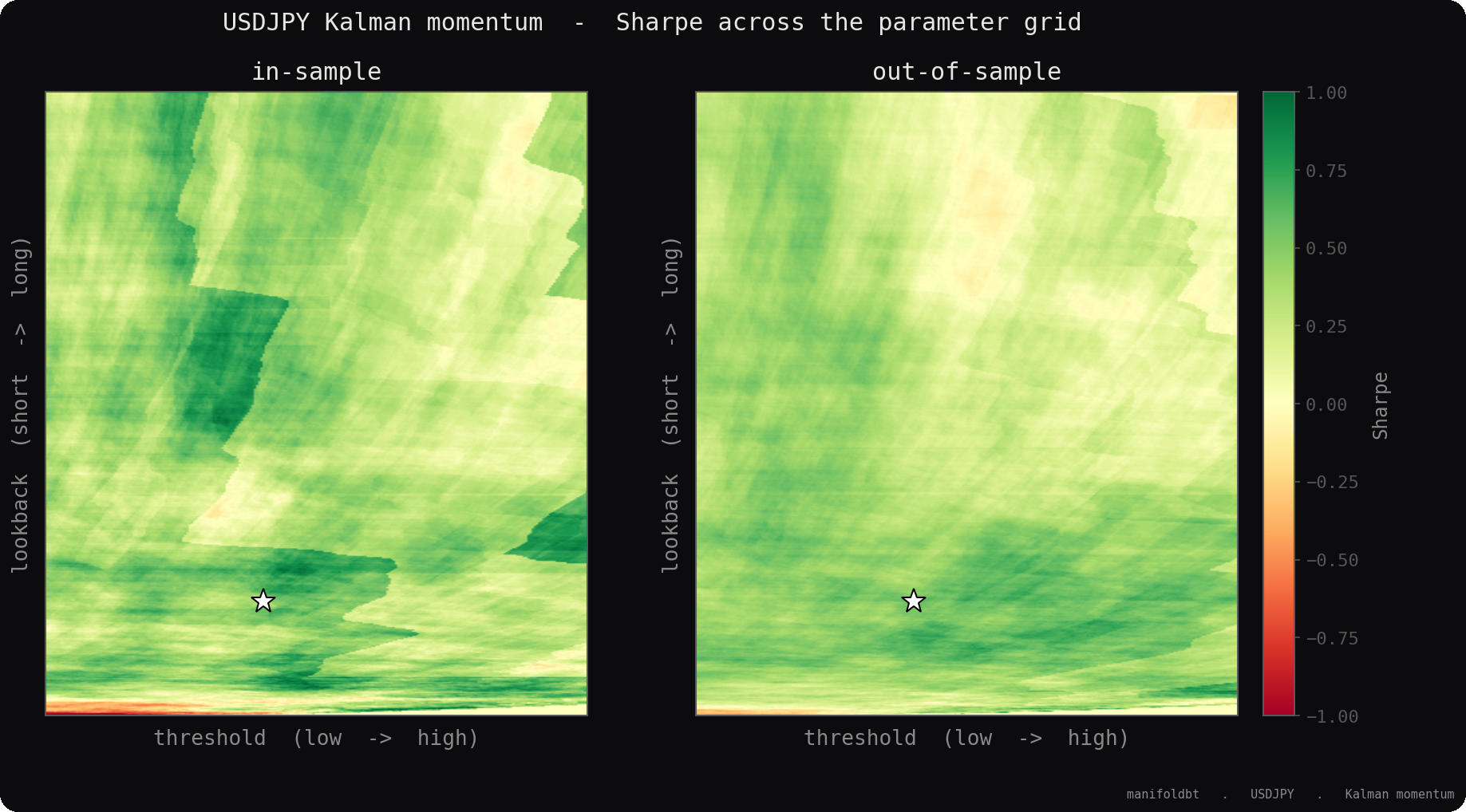
The Sharpe over the parameter grid. The green plateau occupies the same area in-sample and out-of-sample.
The edge forms a broad plateau, in the same place in-sample and out-of-sample. This area is not a collection of distinct strategies, but a family of parameterizations of one edge, which we can treat as correlated estimators of that signal (this is the working hypothesis, which the rest puts to the test). The out-of-sample reproduces the in-sample geography, which confirms the region is real. Only the fine differences inside it are chance.
4. Convergence through pooling
Holding this family of parameterizations, we pool them, several sets run as a single equal-weight portfolio. Which ones, and how many? Not an arbitrary top-N, but a statistical rule. Every set whose smoothed in-sample Sharpe (averaged over its 3×3 grid neighbourhood, so that a set counts as stable only if its neighbours also perform) lies within one standard error of the best. Here, 418 of 784.
The effect of pooling is convergence, visible in one chart, the out-of-sample Sharpe as a function of the number of pooled sets, the band showing where a random choice of N sets lands :
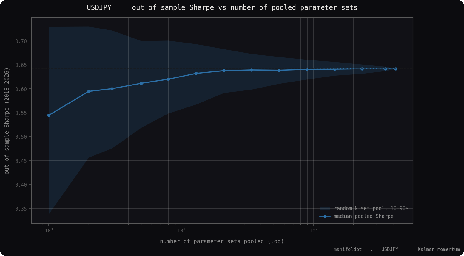
As more sets are pooled, the spread of outcomes closes and the Sharpe converges.
At N = 1, the band spans 0.33 to 0.73. A single set is a draw across that range. As pooling grows, it closes (law of large numbers). By about twenty sets the selection risk drops sharply and the estimate settles at 0.64, above the average single set, pooling cutting volatility while preserving the mean return.
Convergence is not just variance reduction. It raises significance. The CAPM alpha t-stat goes from about 1.4 for the single set to about 2.0 for the pooled region, past the 1.96 threshold. What a single measurement left below the line, the averaged density makes significant.
5. Out-of-sample result
Fixed once on the development window, then run blind on 2018-2026 :
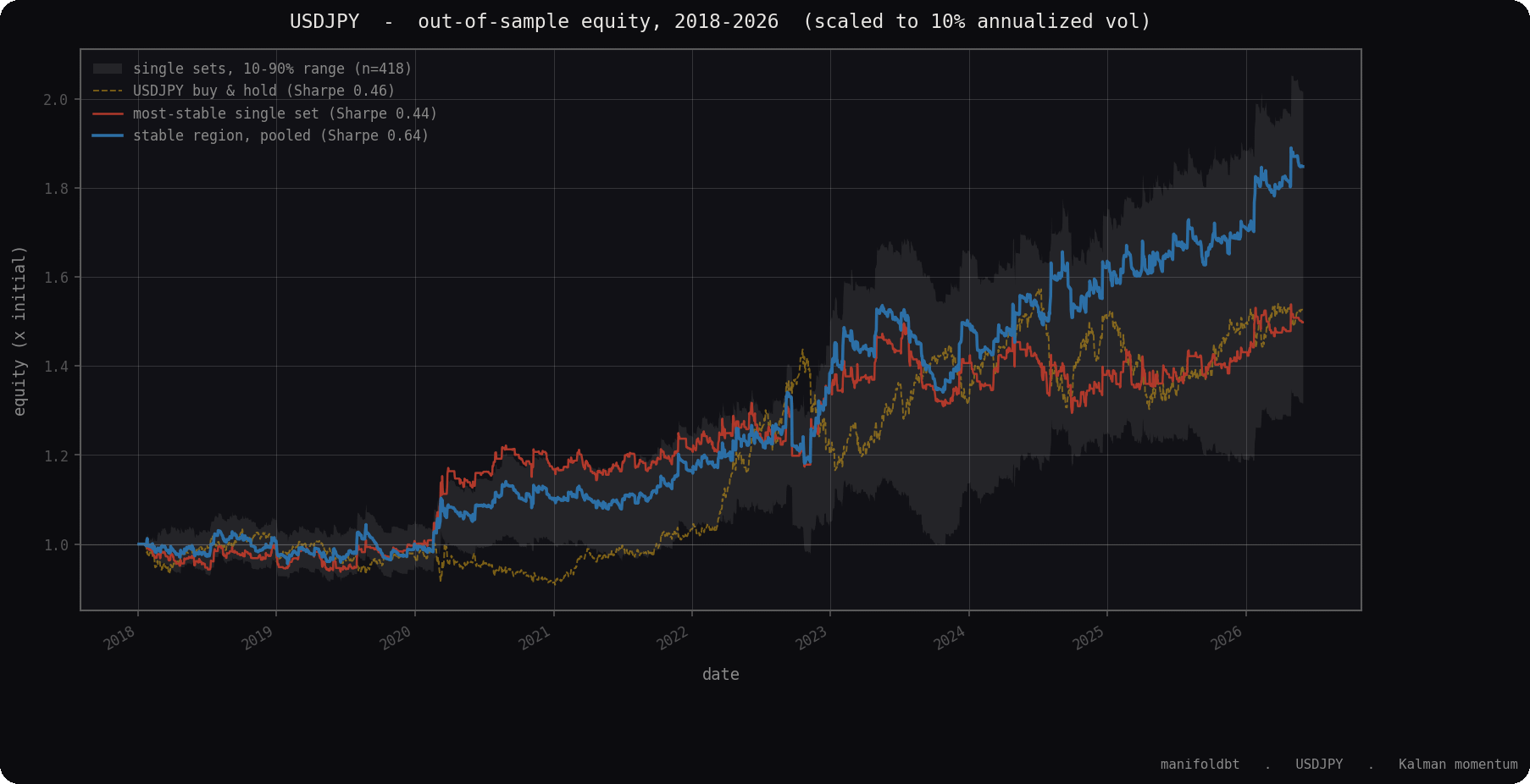
The pooled region (blue) against the most-stable set (red) and buy and hold, all scaled to the same annualized volatility so terminal equity reflects the Sharpe (scaling leaves it unchanged). The grey band shows the spread of individual sets.
Out-of-sample Sharpe (2018-2026)
Most-stable single parameter set : 0.44
Pooled region (418 sets) : 0.64
USD/JPY buy and hold : 0.46
The pooled portfolio beats the disciplined single choice (0.64 versus 0.44), compounding to more at equal volatility, with near-zero beta to the yen and a statistically significant alpha (quantified above). The grey band reflects the spread of individual sets. The blue line is their stable centre, never resting on a single measurement.
Two honesty caveats. First, USD/JPY was selected among several FX pairs. The significance shown does not correct for that asset choice (multiple testing), and the demonstration is about the method, not this particular edge. Second, the backtest already includes minimal fees (0.2 bps). At higher real costs, an FX edge this clean would become marginal. The gain is therefore modest, and that is the point. It is not a source of exceptional return, but a method of estimation.
6. The takeaway
On a single parameter set, the estimate of the signal is noisy and arbitrary. The most reliable one is not the best point, but the average of all the sets the data cannot tell apart. Map the surface, bound the region, average. Do not pick.
This takes a large number of backtests, fast and reproducible. These steps amount to hundreds of thousands of runs, whose purpose is precisely to replace a single measurement with a converged estimate. A backtester that gets you to that verdict quickly is worth more than one that sustains the illusion.
Engine : manifoldbt · GitHub · Discord